 |
Least-Squares Fitting |
 |
Least-Squares Fitting |
![]() The detail of the mathematics given in this page is to be treated as
extra-curricular material.
The detail of the mathematics given in this page is to be treated as
extra-curricular material.
Least-Squares Fitting
Least-squares fitting is an essential element of structure refinement, so some understanding of the concepts involved is needed for a full appreciation of the structure refinement process. However, you do not need a detailed understanding of the mathematics unless you wish to write your own computer programs for least-squares fitting.
Linear Least-Squares
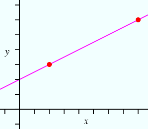
Before considering the complexities of crystallographic least-squares
refinement, it is instructive to consider the simple case of linear least-
squares for the two parameter straight-line function
which may be written in matrix format § as:
| ( y1 ) | = | ( x1 | 1) | ( m ) | ||
| ( y2 ) | ( x2 | 1) | ( c ) |
The parameters of m and c are obtained by inverting the 2 × 2 square matrix and multiplying it by the column matrix in y as shown below:
| ( m ) | = | ( x1 | 1 )−1 | ( y1 ) | ||
| ( c ) | ( x2 | 1 ) | ( y2 ) |
This demonstrates that a simple matrix inversion method can be used to determine values for the two unknown parameters, m and c. The 2 × 2 square matrix used here is an example of a design matrix.
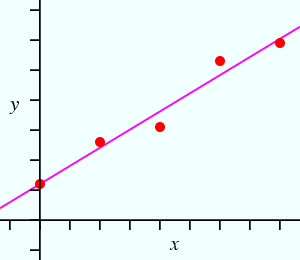
Now suppose we have more observations than parameters as shown in figure B below:
 |
 |
| Figure A | Figure B |
|---|
We can now write 5 equations of the type
| ( y1 ) | = | ( x1 | 1 ) | ( ( |
m c |
) ) |
||
| ( y2 ) | ( x2 | 1 ) | ||||||
| ( y3 ) | ( x3 | 1 ) | ||||||
| ( y4 ) | ( x4 | 1 ) | ||||||
| ( y5 ) | ( x5 | 1 ) |
Any pair of the above equations can yield values for m and c, but the values will depend on which pair of equations is picked, i.e. the values of m and c will not be unique. We might then ask: what are the best/optimum values for m and c? (Note that this makes the tacit assumption that a straight line function provides an appropriate model for the data.) It has proved easy to solve this problem by defining the best values as those for which the function (y(obs) − y(calc)) squared is a minimum: hence the expression least-squares minimization. For the case of our straight line function, this involves minimization of:
| S = | Σ i |
( yi − (m xi + c))2 |
| ( | ∂S
— ∂pj |
)k | = 0 |
| ( | ∂S
— ∂m |
)c | = | 2m | Σ i |
xi2 + 2c | Σ i |
xi − 2 | Σ i |
xi yi | = 0 |
| ( | ∂S
— ∂c |
)m | = | 2m | Σ i |
xi + 2c | Σ i |
1 − 2 | Σ i |
yi | = 0 |
These two linear equations with two unknown parameters may be solved to give the "best" values for m and c directly. The approach may be generalized to the fitting of M parameters with N observations (where M < N) as long as the function is linear in the M parameters.
Iterative Methods
Crystallographic least-squares refinements require a quite different approach, because the functions, whether they be for unit-cell or structure refinement, are very non-linear in all (or nearly all) of the parameters. In consequence, a non-linear least-squares refinement procedure must be used, and for this a numerical iteration process is required. Before explaining non-linear least-squares, a short digression on the subject of iteration is given.
Suppose that we want to know a solution to the equation ƒ(x) = 0, where the function ƒ(x) = y is shown (in magenta) in the figure below:
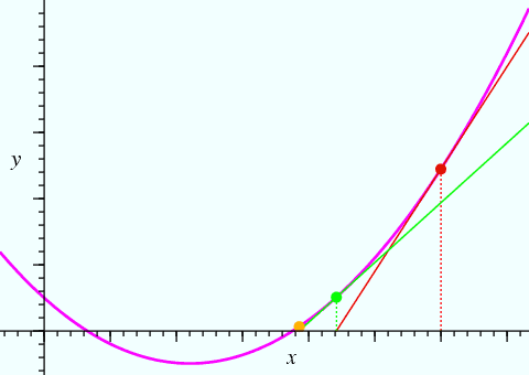
We might guess that one solution to the equation corresponds to the x value of the point shown in red. Newton's method gives an improved value for the solution to the equation using the gradient, dƒ/dx, at this point:
| x2 = x1 − ƒ(x1) / | ( |
dƒ
— dx |
) |
Using this equation, the x value of the point shown in green is obtained. The process can be repeated yet again, and it should be obvious from the figure that the next iteration will give a value of x (indicated by the third point in orange) that is very close to one solution of the equation ƒ(x) = 0.
When considering crystallographic refinements it is important to understand the necessity of iteration, where in general several (or sometimes many) refinement cycles are required to obtain best-fit parameter values, in contrast to the linear least-squares process described earlier, where the results are obtained directly and without the requirement for initial values of the parameters. The figure also illustrates another point. Suppose that the initial value chosen for x was negative: the procedure would still converge, but to a different value of x. In this instance, the alternative value for x is an equally valid solution to the equation ƒ(x) = 0. However, the functions used in crystallography are not as simple as shown here, and poor initial values, e.g. a poor initial crystallographic model, can result in the iterative least-squares refinement converging to a false solution, often called a local minimum. Crystallographers need to be able to spot local minima and escape from them in order to find the global minimum.
Non-linear Least-Squares
It was stated earlier that the function we want to minimise in the Rietveld method is
| Δ = | Σ i |
wi { yi(obs) − yi(calc)}2 |
| ( | ∂Δ
— ∂pj |
)k | = | N Σ i =1 |
{ | 2wi ( yi(obs) − yi(calc)) | ( | ∂yi
— ∂pj |
)k | } | = 0 | [1] |
where N is the total number of observations, i. If there are M parameters, pj, then we have M equations of this type. Supposing that we now have a crystallographic model that is close to satisfying the above equations, but such that parameters in our model differ from those of the true minimum by an amount δpj.
The value of a function at x + Δx given its value at x can be calculated using the Taylor series:
| ƒ(x + Δx) = ƒ(x) + Δx | dƒ(x)
—— dx |
+ | (Δx)2
—— 2! |
d2ƒ(x)
—— dx2 |
+ | (Δx)3
—— 3! |
d3ƒ(x)
—— dx3 |
+ ... |
As the difference Δx tends to
δx tends to zero,
then the higher terms Δxn in
this expansion may be ignored for n > 1.
It is upon this assumption that the
whole process of non-linear least-squares refinement is based. If the
initial crystallographic model is too approximate, then the
assumptions made in the least-squares procedure will not be valid.
As a result of this approximation,
all crystallographic refinements are of an iterative nature.
Applying the Taylor expansion to our multi-parameter function y(calc) gives:
| yi(calc) = yi(p1 ... pM) + | M Σ k=1 |
δpk | ( | ∂yi
— ∂pk |
)j | [2] |
Substituting y(calc) from equation [2] into equation [1] (and rearranging) results in the jth so-called normal equations:
| N Σ i=1 |
M Σ k=1 |
wi δpk | ( | ∂yi
— ∂pk |
)j | ( | ∂yi
— ∂pj |
)k | = | N Σ i=1 |
{ | wi ( yi(obs) − yi(p1 ... pM)) | ( | ∂yi
— ∂pj |
)k | } |
These are more easily visualized in matrix form as shown schematically below:

where A is an M × M symmetric square matrix and
S and V are M × 1 column matrices.
The column matrix S contains the shifts
δpj that will be added
to the parameters as part of the least-squares refinement procedure.
In order to obtain the matrix S, it is necessary to invert the square
matrix A, i.e.
| A(j,k) = | N Σ i=1 |
wi | ( | ∂yi
— ∂pk |
)j | ( | ∂yi
— ∂pj |
)k |
while the elements of the matrix V contain information regarding the observed data:
| V(j) = | N Σ i=1 |
{ | wi ( yi(obs) − yi(p1 ... pM)) | ( | ∂yi
— ∂pj |
)k | } |
From this we can see that if there are problems in inverting the matrix A, then it is our crystallographic model that is at fault and not the data. Furthermore, if the model is good (so that the matrix inverts correctly), but the data are poor, then the calculated shifts to the parameters will be ill-defined.
§ The large brackets used for matrices (and partial derivatives) are difficult to render in standard HTML: stacked round brackets have therefore been used as a replacement. Our apologies for this rather poor alternative.
| © Copyright 1997-2006. Birkbeck College, University of London. | Author(s): Jeremy Karl Cockcroft |