 |
Unit-Cell Refinement |
|
|
Unit-Cell Refinement |
Unit-Cell Refinement
Once an angle-dispersive powder diffraction pattern has been indexed, it may be reduced to a list of hkl and observed 2θ values. This implies that the unit-cell parameters are known approximately; they may then be refined by a least-squares fitting procedure that minimizes the quantity:
| N | |
| Σ | |
| n=1 |
| 2θn(calc) = | 2 sin-1 (λ / 2d) |
| = | 2 sin-1 (λ √{A h2 + B k2 + C l2 + D kl + E hl + F hk} / 2) |
The minimisation function may also include diffractometer calibration constants: for cylindrical samples in transmission geometry the most common additional parameter is the zero error in the 2θ scale, 2θzero, which takes into account the fact the instrumental 180° position does not correspond to the actual incident beam; however you should be aware that this parameter will also tend to compensate for sample displacement errors. For flat-plate samples in reflection geometry a correction for the specimen height displacement can be refined; this has a different functional form to the 2θzero error correction, but over a small range of scattering angle its effect may appear somewhat similar. Even when the specimen height is correct, apparent height displacements may occur when the absorption of the sample is very low (as discussed earlier). Similar comments can be made about sample displacement effects with the cylindrical samples used in transmission geometry. With computer programs that have parameters for both zero error and sample displacement error, only one of these parameters should be refined; unstable refinements are to be expected when both parameters are refined simultaneously.
As with any least-squares refinement, it is a requirement that the number of observations exceeds the number of parameters; thus a greater number of indexed reflections will be required for triclinic than for, say, cubic unit-cell parameter refinement.
A web-based program, identified by the clickable icon
![]() ,
is provided here to demonstrate the refinement of unit-cell parameters.
As with the hkl generating program, we shall be making use of
this program in this and other sections of the course.
(As made available here, this program does not have any facility for
the refinement of sample displacement parameters.)
,
is provided here to demonstrate the refinement of unit-cell parameters.
As with the hkl generating program, we shall be making use of
this program in this and other sections of the course.
(As made available here, this program does not have any facility for
the refinement of sample displacement parameters.)
The least-squares procedure also yields estimated standard deviations (esd's), also known as standard uncertainties (su's), for each of the coefficients A...F of the metric tensor. From these values, esd's on the unit-cell parameters may be obtained, though the equations for calculating them correctly are exceedingly complex. The esd's are a measure of the precision of the refined unit-cell parameters, and not a measure of their accuracy.
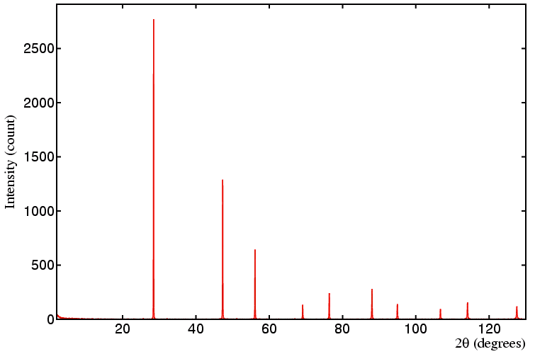
There are several factors that determine the precision of the cell parameters. A few of these will be illustrated with reference to the data set below, which is obtained from a silicon standard run on a well-aligned Bragg-Brentano diffractometer with Cu Kα1 X-ray radiation:
Click each of the icons below to obtain the pre-completed form, which has been filled in with data as described against each icon, and then submit the form:
|
|
|
|
|
|
The first unit-cell refinement should yield an esd value of 0.00016 Å on the unit-cell parameter, the second should give an esd value of 0.00007 Å, and the final esd should be 0.00004 Å. This exercise demonstrates two points: that high-angle data lead to more precise lattice parameters, as do a larger number of data points. However, the "rule" that high-angle data result in more precise unit-cell values should be treated with respect, especially for X-ray data. This is due to the fact that the width of the Bragg reflections at large scattering angles is generally increasing with increasing angle, while at the same time the intensity of the peaks is diminishing due to the effects of X-ray form factors and thermal vibration. The result may be that the positions of the high-angle peaks are determined less precisely than those at intermediate angles, so that no significant improvement in precision is obtained by including poorer quality high-angle data.
Although refinement of the unit-cell parameters should be relatively straightforward, problems may occur. The most common is for reflections to be misindexed or for the wrong 2θ values to be used. Some software packages will be able to cope with this, while others may not. Typical effects are demonstrated below, where deliberate errors have been introduced into the input data:
|
|
|
|
In the first refinement, the program is able to spot the error and reject the reflection. However, in the second refinement the combination of the two errors simply results in a bad fit since the program has failed to reject the two peaks with the wrong hkl indices. The refinement is clearly duff since all of the Δ 2θ / σ values are unacceptable; consequently the esd's on the cell parameters are very large.
|
© Copyright 1997-2006.
Birkbeck College, University of London.
|
Author(s):
Jeremy Karl Cockcroft Martin Vickers |